TUTORIAL IN DEA
1. Historical Background and Philosophy
Efficiency analysis has always interested researchers because of the relative
difficulty encountered in assessing the performance of a firm or an organization. Using an engineering –like approach,
Farrell (1957) attempted to measure the efficiency of a unit of production in the single input-single output case.
Farrell’s study involved the measurement of price and technical efficiencies and the derivation of the efficient production
function
Farrell applied his model to estimate the efficiency of the US agriculture relative to other countries. However, he failed in providing a way to summarize all various inputs and outputs into a single virtual input and single virtual out
Charnes, Cooper and Rhodes extended Farrell’s idea and proposed a model that generalizes the single-input, single-output ratio measure of efficiency of a single Decision-Making Unit (DMU) in a multiple-inputs, multiple outputs setting. A DMU is a entity that produces outputs and uses up inputs. In banking, a bank branch constitutes a DMU. The technical efficiency of a DMU is computed using the engineering-like efficiency measure of efficiency as ratio of virtual output produced to virtual input consumed:

As for the weights used in the transformation of the vectors of inputs and outputs into two single virtual scalars, the DEA model allows each DMU to choose the set of multipliers (weights) m
o and n
o that permits it to appear in the best light. The efficiency score obtained is also relative to a sample of DMUs under analysis since the set of weights has to be feasible for other units and none of these units should have an efficiency score greater than one.
In contrast to Regression Analysis, which gives us an average profile of DMUs under analysis (see figure 1), DEA yields a piecewise empirical external production surface that, in economic terms represents the revealed best practice production frontier (or envelope). By projecting each unit onto the frontier, it is possible to determine the level of inefficiency by comparison to a single reference unit or a convex combination of other reference units. The projection refers to a virtual DMU which is a convex combination of one or more efficient DMUs. Thus, the projected point may itself not be an actual DMU. The link can be made with Markowitz’s portfolio efficient frontier (1953) idea in which DMUs are supposed to be in some way divisible and that a benchmark, which is a convex combination of other efficient DMUs, can virtually exist. The inefficient DMU is, therefore, supposed to emulate the benchmark’s practices in order to become efficient.
 Back to table of contents Back to table of contents
2. Basic Models in DEA
The first standard DEA model as proposed by Charnes, Cooper, and
Rhodes (1978), in ratio form is expressed as follows:
Model 1: CCR input-oriented ratio form
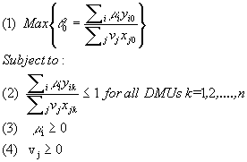
The parameters used in model 1 are:
q 0 = the efficiency score of the
DMU 0 under analysis;
n = number of DMUs under analysis;
I = number of outputs;
J = number of inputs;
Yk = {
y1k, y2k,...,yik,…,yIk}
is the vector of outputs for DMU k with yik being the value of output i for DMU k;
Xk = {
x1k, x2k,...,xjk,…,yIk}
is the vector of inputs for DMU k with xik being the value of input j for DMU k;
m
and n
the vector on multipliers respectively set on Yk and Xk where m
i, n
j = the respective weights for output i and for input j;
Given a set of J Decision Making Units (branches), the model determines for each DMU0
the optimal set of input weights  and output weights and output weights
 that maximizes its efficiency score eo. that maximizes its efficiency score eo.
Charnes, Cooper and Rhodes (1981) defines efficiency by reference to the orientation chosen:
- In an output oriented model, a DMU is not efficient if it is possible to augment any output
without increasing any input or decreasing any other output.
- In an input oriented model, a DMU is not efficient if it possible to decrease any input without
augmenting any other input and without decreasing any output.
A DMU will be characterized as efficient if and only if neither (i) or (ii) occurs. A score less than
one means that a linear combination of other units from the sample could produce the vector of outputs using a smaller
vector of inputs. Mathematically, a DMU is termed efficient if its efficiency rating qo obtained from the DEA model is equal to one. Otherwise, the DMU is considered inefficient.
An attempt to impede false technical efficiency was made through the introduction of the small
non-archimedian infinitesimal e to prevent DMUs from giving zero weights to factors that manage poorly (Charnes et al 1981). The actual set of constraints reflecting this is:

With  is a vector of unities. is a vector of unities.
The above fractional programming model is clearly non linear. Using the linear transformation of Charnes and Cooper (1962), namely , we obtain the model CCR-D. , we obtain the model CCR-D.
Model 2: the CCR-Dual input oriented
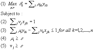
The associated primal model is (as the terminology switched since the BCC model in 1984):
Model 3: CCR-Primal
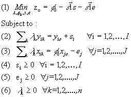
Model 2 can be interpreted as follows. Any particular DMU "o" has the latitude to
choose the set of weights that maximize its efficiency relative to other DMUs of the sample provided that no other DMU
or convex combination of DMU could achieve the same output vector with a smaller input vector. Model 3 (the primal)
visualizes more directly the previous statement. A DMU "o" is efficient if there exists no convex combination
of DMUs  that produces a higher level of output than the actual
one produced by DMU o, yio. without consuming any more input or decreasing the amount produced
of other outputs. The parameter f
o refers to amount of possible proportional reduction in the vector of input Xo
while maintaining the same level of outputs. This reduction is applied simultaneously to all inputs and results
in a radial movement toward the envelopment surface. Finally, in order to adjust DMU "o" to its projection
on the frontier, slacks si (referring to shortage in output production for the specific output i) and slacks
ej ( referring to excessive use of input j) are introduced. The primal necessitates thus a two-stage process
to determine the projection point for DMU "o". First, the amount of maximal possible proportional shrinkage
in input, f
*o , is determined. Then, the model identifies individual slack that are necessary in
order to drive "o" towards its projection on the frontier. Notice that in order to be efficient, both
f
*o must be equal to 1 and all slacks must be null. that produces a higher level of output than the actual
one produced by DMU o, yio. without consuming any more input or decreasing the amount produced
of other outputs. The parameter f
o refers to amount of possible proportional reduction in the vector of input Xo
while maintaining the same level of outputs. This reduction is applied simultaneously to all inputs and results
in a radial movement toward the envelopment surface. Finally, in order to adjust DMU "o" to its projection
on the frontier, slacks si (referring to shortage in output production for the specific output i) and slacks
ej ( referring to excessive use of input j) are introduced. The primal necessitates thus a two-stage process
to determine the projection point for DMU "o". First, the amount of maximal possible proportional shrinkage
in input, f
*o , is determined. Then, the model identifies individual slack that are necessary in
order to drive "o" towards its projection on the frontier. Notice that in order to be efficient, both
f
*o must be equal to 1 and all slacks must be null.
Consequently, the conditions to be efficient are equivalently:
- A DMU is efficient if and only if
- f
*o=1
- si=ej=0 for all i=1,2,…,I and j=1,2,…,J
2- a DMU is efficient if and only if q
*o=f
*o=1
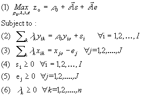
The primal and dual of the CCR output-orientation are given respectively by model 4 and model 5.
Model 4: CCR-Primal output oriented
Model 5: CCR-Dual Output oriented
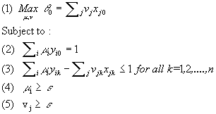
Analogous interpretations to those in the case of input-oriented model can be given.
However, the CCR model does not accomodate returns to scales. Banker, Charnes, and Cooper (1984) suggested the BCC model to cope with this issue. The primal and dual versions of the BCC model are respectively given by model 6 and model 7.
Model 6: BCC-Primal input oriented
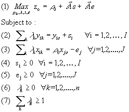
Model 7: BCC-Dual input oriented
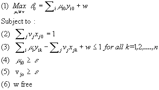
The main distinction between the BCC and the CCR model is the introduction of the parameter w.
w relaxes the constant returns to scale condition by not restricting hyperplanes defining the envelopment surface to go
through the origin (Ali 1994). See §1.3.3 for a graphical representation of the above statement.
The two other basic models in DEA (that are not covered in this paper) are the additive
model (Charnes et al 1985) and the multiplicative model (Charnes et al 1983).
In any case, DEA can be viewed as a projection mechanism of a multi-input, multi-output entity
onto an envelopment surface. Thus, for any DMU "o" characterized by the output-input vector
(Yo,Xo):

As each DMU is allowed to put high weights on factors m
r0 and n
i0 that it handles the best, this may lead to abnormalities and huge discrepancies among the various
multipliers. More advanced models worked thus on introducing more control by imposing bounds on multipliers given
by the constraints:

W 1 and
W2 are "assurance regions" defined by any restrictions imposed
on multipliers. Such restrictions can be ratio constraints on m
i0 and n
j0 or can be of an absolute value type (e.g. 0.3£
m
i0£
0.5). The efficiency score for any DMU k is also constrained to be less than 1
(as stated by equation (2)).
Bounds on weights are imposed in order to ensure that no false efficiency can be achieved
by putting a huge weight on one or few factors (inputs and outputs) and assigning a zero weight to all other factors. In
fact, a logical trade-off exists between each pair of outputs and each pair of inputs in term of their relative importance
to the decision maker. Such tradeoffs are the references that are used to generate W
1 and W2 (the set of restrictions imposed
on multipliers). For instance, one may consider that processing a loan is roughly between two and three times as important as processing a visa advance. Mathematically, these constraints can be expressed as follows:
 . .
Many techniques have been proposed for expressing judgements in DEA and are
presented in §1.3.4.
 Back to table of contents Back to table of contents
3. Inputs and Outputs
Traditional DEA models, as outlined by Charnes et al (1978) implicitly assumed
that factors
(inputs and outputs) are discretionary, which means that they are controllable and can be set up by the decision-maker.
However, in many realistic situations, variables are exogenous and non discretionary. In the case of bank branch efficiency,
most outputs are non discretionary. For instance, a branch can rarely control the number of deposits processed or the
number of RRSPs sold. Banker and Morey (1986) proposed a methodology to include non discretionary variables in DEA.
This is mainly done by maximizing (minimizing) only discretionary outputs (inputs) in the linear program (LP) model.
DEA can also integrate categorical variables (non continuous variables) in the LP model such as
discrete ordinal variables (dummy variables). Other authors have analyzed the issue using categorical variables by proposing
alternate formulation of the LP model (Cook et al 1993). Several authors have proposed different formulations that account for
ordinal variables (Cook, Kress and Seiford 1996).
Consequently, DEA embodies all different types of variables, whether they are discretionary or non
discretionary, categorical (ordinal) or continuous.
 Back to table of contents Back to table of contents
4. Orientations in DEA
DEA offers three possible orientations in efficiency analysis (Charnes et al 1994):
- Input-oriented models are models where DMUs are deemed to produce a given
amount of outputs with the smallest possible amount of inputs. (inputs are controllable)
- Output-oriented models are models where DMUs are deemed to produce with
given amounts of inputs the highest possible of outputs. (outputs are controllable)
- Base-oriented models are models where DMUs are to deemed to produce the
optimal mix of inputs and outputs. (both inputs and outputs are controllable)
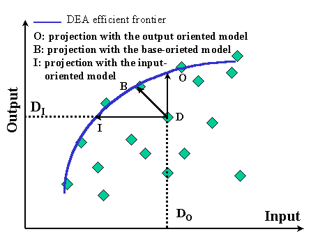
Figure 2 describes the simple case of a single-input single output production system. Point I
constitutes the benchmark for inefficient DMU D in the input-oriented model. The relative efficiency of D is given by
the ratio of distances  . Point O is the projection of D in the
output-oriented model. The relative efficiency of D is then . Point O is the projection of D in the
output-oriented model. The relative efficiency of D is then  .
Finally, point B is the base-projection of D in the base oriented model. .
Finally, point B is the base-projection of D in the base oriented model.
Figure 2 Projection of an inefficient unit on the frontier with the three
possible orientation of a DEA model
 Back to table of contents Back to table of contents
5. Returns to Scale Version
The second feature of a DEA model is the structure of its returns to scale. This
can be either a Constant Returns to Scale structure (CRS), or a Variable Returns to Scale (VRS). In the case of a CRS, it is
assumed that an increase in the amount of inputs consumed would lead to a proportional increase the amount of outputs
produced. In the VRS, the amount of outputs produced is deemed to increase more or less than proportionally than the
increase in the inputs.
The CRS version is more restrictive that the VRS and yields usually to a fewer number of efficient
units and also lower efficiency scores among all DMUs. This is due to the fact that the CRS is a special case of the VRS model. As indicated earlier, the VRS model is given by:
For each DMU "o"
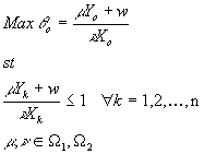
m
and n
are the set of weights applicable respectively to the vector of outputs Yo and that of inputs Xo. W1 and W2 denote the "assurance regions" restricting m
and n
.
The CRS version corresponds to the special case where w is constrained to be zero. The optimal
solution of the CRS model qcrs* thus is by construction lower than
qvrs* of the VRS model.
Figure 3: Computing efficiency in the VRS and CRS models
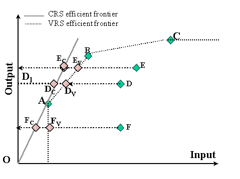
Figure 3 illustrates of the previous argument. It depicts the case of a single-input single output
system. Using an input-orientation, the VRS envelope is formed by DMUs A, B, and C. The CRS envelope is however
formed by the straight line originating from O and going through point A. Although A, B, and C are efficient with the VRS
model, only A appears efficient in the CRS model. Even DMUs that are found inefficient in the VRS model (E,D, and F)
experience a drop in their efficiency rating with the CRS model..
For instance,  , the efficiency score of
point D under a VRS evaluation is given by , the efficiency score of
point D under a VRS evaluation is given by  . This measure is larger
than . This measure is larger
than  , the CRS efficiency score of DMU D, which is given by , the CRS efficiency score of DMU D, which is given by
 . .
 Back to table of contents Back to table of contents
6.Expressing Judgements in DEA
The original CCR (1978, 1981) and BCC (1984) models were originally
unbounded models as no restrictions were imposed on multipliers. However, a score of 100% efficiency can be
achieved through several different means. A DMU can spread its weights equally among the various inputs and outputs;
such DMUs can be referred to as generalists. Alternatively, a DMU can put a huge weight on one or few factors
and assign a zero or very small weights to other factors. Such DMUs can be referred to as mavericks.
However, the complete flexibility of DEA may induce undesirable consequences, since any
particular DMU can appear efficient in ways that are difficult to justify. The DEA model gives often excessively high or
low values to multipliers in an attempt to drive the efficiency score as high as possible. Charnes et al (1994) cite three
situations where additional control on multipliers is needed:
The analysis ignores additional information that can not be directly incorporated into the
model or that contradicts expert opinions
Management has strong preferences about the relative importance of different factors
When the number of factors is relatively large compared with the number of DMUs under
analysis, the model fails to discriminate and most DMUs appear efficient.
Consequently, additional efforts were put toward further resticting weights in DEA. Charnes et
al (1989) used a cone-ratio formulation that restricts the virtual dual multipliers to some closed convex cones. Thompson et al (1990) developed a similarly motivated approach, based on the so-called Assurance Region models, that focuses on imposing bounds on ratio of multipliers. Dyson and Thanassoulis (1989) and Cook et al (1991) proposed techniques involving enforcing upper and lower bounds on multipliers. Finally, Beasley and Wong (1991) suggested restricting the proportion of multipliers m
i, n
j compared to the total amount of standard outputs (inputs) as follows:
 and and 
A-, A+, B-, and B+ denote respectively the lower and upper bounds on the ratio of multipliers.
 Back to table of contents Back to table of contents
7. Strengths and Weaknesses of DEA
DEA provides a comprehensive picture of organizational performance. It seems
to be a particularly appropriate tool for financial services organizations. This is partially due to the fact that a multitude of
subjective factors affect the service quality and the productivity of a service business. It is also difficult to find a commonly
agreed upon functional form relating inputs consumed to outputs produced.
Depending on the orientation of the problem (input-oriented, output-oriented or base model),
DEA presents three extremely useful features (Charnes et al 1994):
- it characterizes each DMU by a single efficiency score;
- by projecting inefficient units on the efficient envelop, it highlights areas of improvements
for each single DMU;
- it facilitates making inferences on the DMUs’ general profile.
Charnes et al (1994) give a complementary list of other advantages of DEA:
- the possibility of handling multiple inputs and outputs stated in different measurement units;
- the focus on a best-practice frontier, instead of on population central-tendencies. Every unit is compared to an efficient unit or a combination of efficient units. The comparison, therefore, leads to sources of inefficiency of units that do not belong to the frontier;
- no restrictions are imposed on the functional form relating inputs to outputs.
These characteristics have made DEA a popular method in efficiency assessment.
However, standard DEA models include some inherent limitations. The same characteristics that make DEA a powerful tool can also create problems. An analyst should keep these limitations in mind when choosing whether or not to use DEA. Since DEA is an extreme point technique, noise (even symmetrical noise with zero mean) such as measurement error can cause significant problems. Since DEA is a non-parametric technique, statistical hypothesis tests are difficult and are the focus of ongoing research. Since a standard formulation of DEA creates a separate linear program for each DMU, large problems can be computationally intensive. Some packages are available which facilitate the processing of large amounts of data.
Traditional DEA analysis has other limitations (Athanasspoulis 1991):
- limitations in aggregating different aspects of efficiency, especially in the case where DMUs perform multiple activities.
- insensitivity to intangible and categorical components (for instance, the service quality in a bank branch setting).
Another problem relates to the difficulty of mixing different dimensions of the analysis. Consider a DMU performing two different functions. The DMU can be found efficient in the first function and extremely inefficient in the second function. For instance, bank branches are a single platform that management uses to sell financial services to customers as well as providing more traditional banking services such as processing deposits or loans. In other words, it is difficult to study the sales efficiency and the service efficiency of the branch in the same time. A similar problem would be studying the productivity and the profitability of the branch simultaneously as the first dimension implies using operational inputs and outputs and the second one implies using financial ones. Since relevant inputs and outputs for each dimension are not directly comparable, the analyst would have to run two DEA models, a productivity model and a profitability one. Then, the problem of compromising both models’ findings arises. Cook et al (1998) developed a methodology aimed at evaluating sales and service efficiencies in bank branches. Their work came as an extension to Beasley’s (1991) attempt to evaluate simultaneously research and teaching efficiencies for various university department.
Finally, DEA is intended for estimating the relative efficiency of a DMU but it does not specifically address absolute efficiency. In other words, it tells how well the DMU is doing compared to the peers (set of efficient units), but not compared to a theoretical maximum. The two major inconveniences resulting from this are:
- the impossibility of ranking efficient units; indeed all efficient units have an efficiency score of 100%;
- from a managerial point of view, it may be more useful to compare branches to a frontier of absolute best performance. Therefore, the analyst would be able to better detect, for example, a bank branch network’s true inefficiencies. In fact, one might argue that efficient units may not be efficient enough and that the created frontier does not reflect the real potential of the branch network. It must be emphasized again, that the setting where DEA is most useful are those where it is not possible to loosely generate industry standards, hence an absolute frontier is not possible.
Finally, there is no specific methodology for predicting or testing the appropriateness of a set of factors in an efficiency study. A DEA model can indicate out of a given set of factors, how efficient a specific DMU is, and what its efficiency score is. It does not indicate, however, whether the chosen factors are the right ones to use.
 Back to table of contents Back to table of contents
8. Future research directions in DEA
As DEA gains higher acceptance among practitioners and academicians as a useful technique for evaluating efficiency, several inconsistencies and pitfalls have appeared in the standard DEA models. Development in DEA was stimulated by problems that arose in the process of applying the technique. Moreover, many felt the need to bridge the gap between DEA and other disciplines such as statistics and economics. This has motivated a whole stream of research on specific aspects of DEA among which we can list stochastic DEA, sensitivity analysis, window analysis and integrating DEA and regression models.
As such, DEA have people looked for further validation of the technique by attempting to give stochastic attributes to DEA models. Banker (1993) proved that the efficient frontier corresponds to the maximum-likelihood estimates of the stochastic parametric frontier, thus giving more legitimacy to DEA efficiency rating.
Sensitivity Analysis is also a new rising field in DEA. It aims to test the extent to which results may vary with perturbations in data. Charnes et al (1985) first evaluated the stability of DEA scores to changes introduced to a single output. O’Neill et al (1996), using an index based on Andersen and Petersen’s (1993) superefficiency measure, evaluated the effect of dropping one DMU from the reference set. Seiford and Zhu (1996) studied the sensitivity of DEA models to simultaneous changes in all the data.
Window analysis is another growing field. It pays attention to the temporal evolution of efficiency rating for evaluating how consistent these ratings are. We can quote herein the study by Charnes et al (1985b) on measuring the efficiency overtime of maintenance units in the U.S. air forces.
Other authors have focused on statistical properties of DEA and compared performances assessment with both techniques. Thanassoulis (1993) proved that DEA yields better efficiency estimates than traditional regression models in an application to hospital units. A similar study was conducted by Bowlin et al (1985). Finally, a growing and related area in DEA is stochastic DEA, which strives to adapting DEA models to the stochastic nature of the data .
 Back to table of contents Back to table of contents
Back to Home
|